In this post I will present the speed sensorless control of PMSM. Before You start reading this article please read the following posts, because these articles are related to this topic and I don't detailing here again:
The model of the PMSM is nonlinear, to linearise the system I used the state feedback linearisation. The states can be measured or estimated. In this blog I will present a sensorless solution using the extended Kalman filter.
State estimation
For the motor model linearisation I need to know the direct axis, quadratic axis current and the speed of the rotor.
It has the following system:
$$x_{k+1}=Ax_k+Bu_k+Ew\\y=Cx_k+Du_k\tag{1}$$
Where the states are:
$$\left[\begin{array}{c} i_d \\ i_q \\ \omega_r \\ \theta \\ T_L \end{array}\right]\tag{2}$$
Using the $3-8$ equations from the Dynamic model of a PMSM post, I can write the state space model of the PMSM, also I assume that the changes of the mechanical torque is small or it is constant.
$$A
= \begin{bmatrix} -\frac{R}{L_d} & \frac{L_qP\omega_r}{L_d} & 0 & 0 & 0\\ -\frac{L_dP\omega_r}{L_q} & -\frac{R}{L_q} & -\frac{PL_m}{L_q}
& 0 & 0 \\ 0 & \frac{3}{2}\frac{P}{J}\left(L_m+\left(L_d-L_q\right)i_d\right) & -\frac{B}{J} & 0 & -\frac{1}{J}\\ 0 & 0 & 1 & 0 & 0\\0 & 0 & 0 & 0 & 0\end{bmatrix}\tag{3}$$
$$B= \begin{bmatrix}\frac{1}{L_d} & 0 \\ 0 & \frac{1}{L_q} \\ 0 & 0\\ 0 & 0\\ 0 & 0\end{bmatrix}\tag{4}$$
The model can be discretized by using the following approach:
$$A_d=e^{AT} \approx I+AT\tag{5}
$$$$B_d=\int_0^T e^{At}B dt \approx BT\tag{6}$$
The discretized discrete state space system matrices is as follows:
$$A_k
= \begin{bmatrix} 1-T_s\frac{R}{L_d} & T_s\frac{L_qP\omega_r}{L_d} & 0
& 0 & 0\\ -T_s\frac{L_dP\omega_r}{L_q} & 1-T_s\frac{R}{L_q} &
-T_s\frac{PL_m}{L_q}
& 0 & 0 \\ 0 &
T_s\frac{3}{2}\frac{P}{J}\left(L_m+\left(L_d-L_q\right)i_d\right) &
1-T_s\frac{B}{J} & 0 & -T_s\frac{1}{J}\\ 0 & 0 & T_s & 1
& 0\\0 & 0 & 0 & 0 & 1\end{bmatrix}\tag{7}$$
$$B_k= \begin{bmatrix}\frac{T_s}{L_d} & 0 \\ 0 & \frac{T_s}{L_q} \\ 0 & 0\\ 0 & 0\\ 0 & 0\end{bmatrix}\tag{8}$$
and the Jacobian matrix is:
$$G_k=\begin{bmatrix} 1-T_s\frac{R}{L_d} & T_s\frac{L_qP\omega_r}{L_d} & T_s\frac{L_qPi_q}{L_d}
& 0 & 0\\ -T_s\frac{L_dP\omega_r}{L_q} & 1-T_s\frac{R}{L_q} &
-T_s\frac{PL_m+L_dPi_d}{L_q}
& 0 & 0 \\ T_s\frac{3}{2}\frac{P}{2J}\left(L_d-L_q\right)i_d &
T_s\frac{3}{2}\frac{P}{J}\left(L_m+\left(L_d-L_q\right)i_d\right) &
1-T_s\frac{B}{J} & 0 & -T_s\frac{1}{J}\\ 0 & 0 & T_s & 1
& 0\\0 & 0 & 0 & 0 & 1\end{bmatrix}\tag{9}$$
Filter tunning
I used an AC6 Vector Control for an interior Permanent Magnet Synchronous Motor (PMSM) simulink model to simulate and tune the estimators R,Q covariance matrices:
 |
| Figure 1. |
$$Q=diag\left(\begin{array}{c} 1e-3 & 1e-3 & 1e-1 & 1e-9 & 1e-1\end{array}\right)\\R=diag\left(\begin{array}{c}1e3 & 1e3\end{array}\right)\tag{10}$$
the estimated speed is hence:
 |
| Rotor speed |
Linear Quadratic Regulator
I already wrote a short introduction about the LQR, now I will present only the results. As I mentioned before, to control the system I need to know only the currents and the rotor velocity, so I have the following states:
$$\left[\begin{array}{c} i_d & i_q & w_r\end{array}\right]\tag{11}$$
In this case the state space model is as follows:
choosing the LQR state and input weighing matrices in this way:
$$R=\left[\begin{array}{c} 1e-8 & 1e-8 \end{array}\right]\\Q=\left[\begin{array}{c} 1e1 \end{array}\right]\tag{15}$$
and the horizon to 2, the simulation result is the following:
$$\left[\begin{array}{c} i_d & i_q & w_r\end{array}\right]\tag{11}$$
In this case the state space model is as follows:
$$A_k
= \begin{bmatrix} 1-T_s\frac{R}{L_d} & T_s\frac{L_qP\omega_r}{L_d} & 0 \\ -T_s\frac{L_dP\omega_r}{L_q} & 1-T_s\frac{R}{L_q} &
-T_s\frac{PL_m}{L_q} \\ 0 &
T_s\frac{3}{2}\frac{P}{J}\left(L_m+\left(L_d-L_q\right)i_d\right) &
1-T_s\frac{B}{J}\end{bmatrix}\tag{12}$$
$$B_k=
\begin{bmatrix}\frac{T_s}{L_d} & 0 \\ 0 & \frac{T_s}{L_q} \\ 0
& 0\end{bmatrix}\tag{13}$$
$$C=\left[\begin{array}{c} 0 & 0 & 1\end{array}\right]\tag{14}$$
$$D=[0]$$
$$C=\left[\begin{array}{c} 0 & 0 & 1\end{array}\right]\tag{14}$$
$$D=[0]$$
choosing the LQR state and input weighing matrices in this way:
$$R=\left[\begin{array}{c} 1e-8 & 1e-8 \end{array}\right]\\Q=\left[\begin{array}{c} 1e1 \end{array}\right]\tag{15}$$
and the horizon to 2, the simulation result is the following:
 |
| Results |
Error between the reference speed and the simulated speed using the LQR controller
The error between the reference and simulated value using the ac6_example
As you can see, in the LQR the error is between 1 and -1.5 which is better than the other controller. Still there are possibilities to reduce the error by increasing the number of the horizon and changing the weight matrices.
Here is another result:
Finally, I can put together the estimator and the controller, so I will end up with the following simulink model:
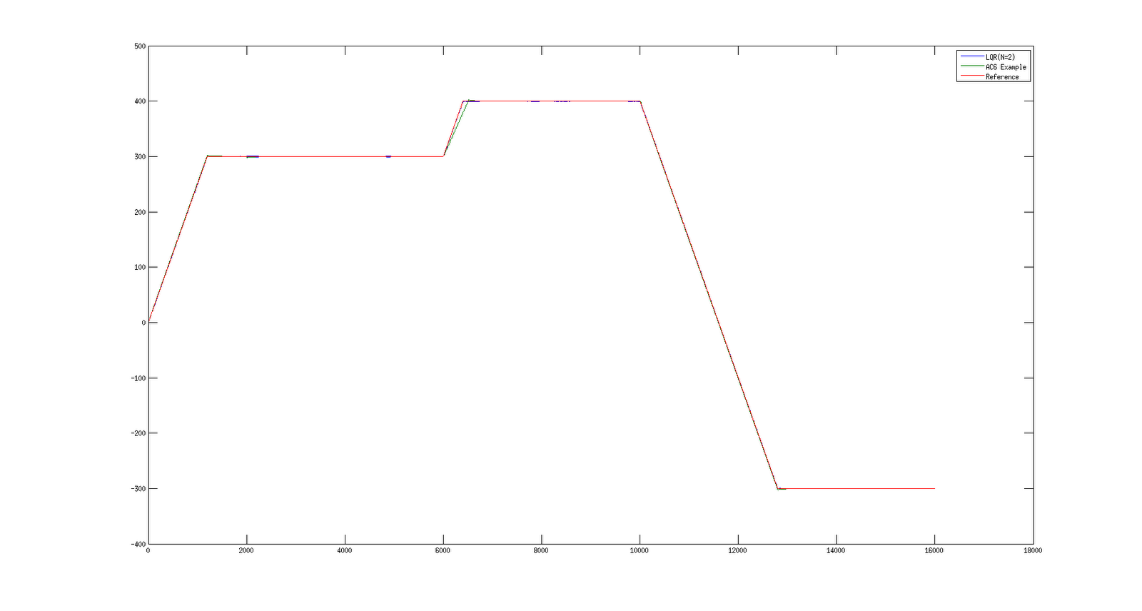
And the result by choosing N=2,


 |
| LQR rotor speed error(N=2) |
 |
| Rotor speed error |
Here is another result:
 | |
| LQR rotor speed error(N=10) |
 | |
| EKF with LQR |
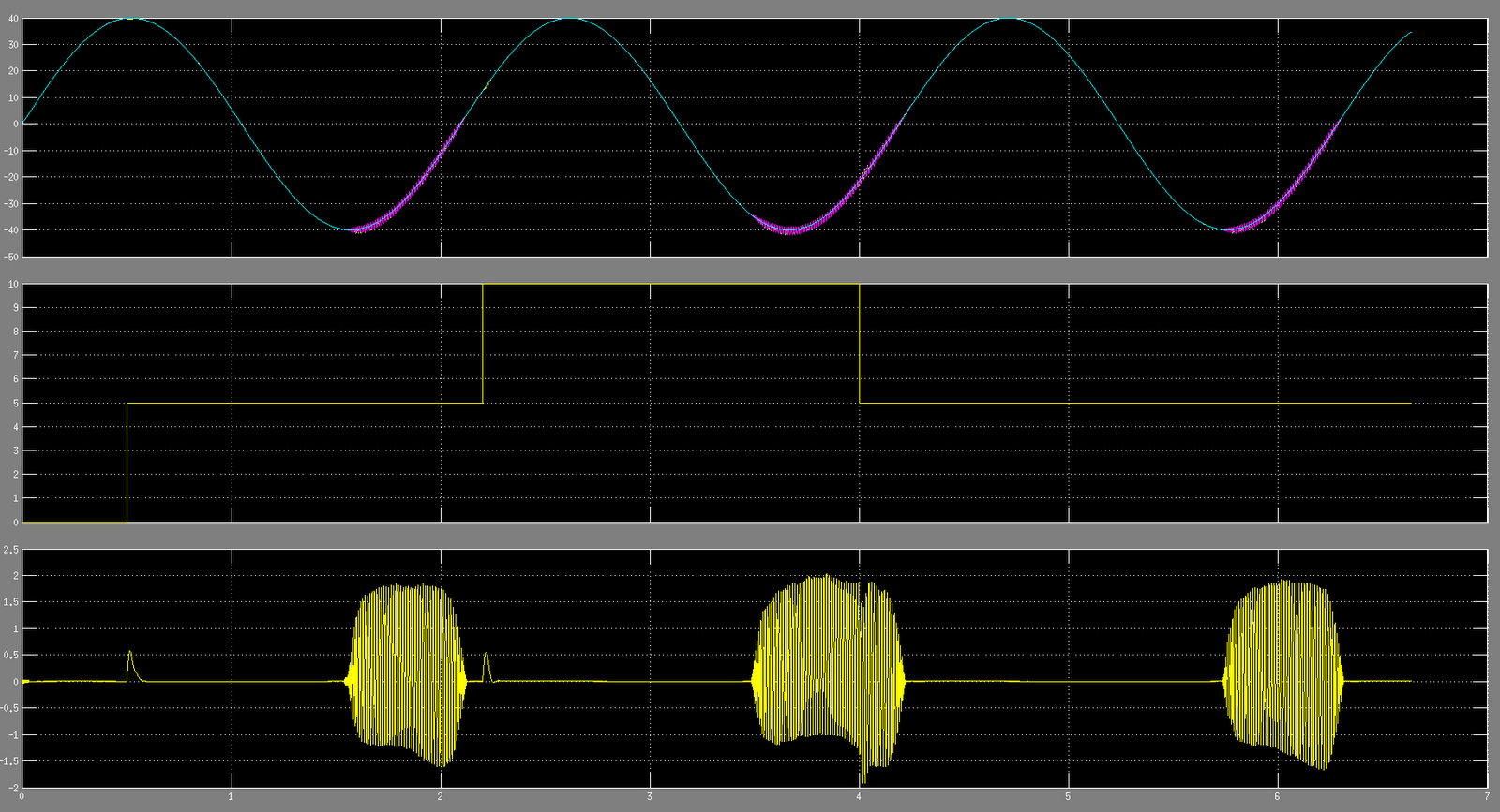
The first subplot is the reference speed and the measured speed, the second is the mechanical torque and the third is the error between the reference and the measured signal.

No comments:
Post a Comment