System Controlling

Sunday, November 18, 2012

Model predictive control of brushed DC motor

Motor model

The state space model of a brushed DC motor as follow:
$$A =\left[ {\begin{array}{cc} -\frac{R_{a}}{L_{a}} & -\frac{K_{e}}{L_{a}} &  0 \\ \frac{K_{m}}{J} & -\frac{b}{J} & 0 \\ 0 & 1 & 0 \end{array} } \right] B=\left[ {\begin{array}{cc} \frac{1}{L_{a}} \\ 0 \\ 0 \end{array} } \right] C=\left[ {\begin{array}{cc} 0 \\ 1 \\ 0 \end{array} } \right] D=\left[ {\begin{array}{cc} 0 \end{array} } \right]\tag{1}$$
As you can see, I assumed that the torque is zero. 
Where the states are:
$$\dot{x(t)} =\left[ {\begin{array}{cc} \frac{di}{dt} \\ \frac{d\omega}{dt} \\ \frac{d\theta}{dt} \end{array} } \right]\tag{2}$$

Controller design


I already introduced the MPC controller, please read that first before you continue to read this blog. 
The first step is to determine the Toeplitz matrix:
$$\begin{bmatrix}x_{k+1|k} \\ \vdots \\ x_{k+N_c|k} \\ x_{k+N_c+1|k} \\ \vdots \\ x_{k+N|k} \end{bmatrix}=\begin{bmatrix}\Phi \\ \vdots \\ \Phi^{N_c} \\ \Phi^{N_c+1} \\ \vdots \\ \Phi^N \end{bmatrix}x_k + \begin{bmatrix}\Gamma \\ \vdots \\ \sum_{i=0}^{N_c-1} \Phi^{i} \Gamma\\ \sum_{i=0}^{N_c}\Phi^{i} \Gamma\\ \vdots \\ \sum_{i=0}^{N}\Phi^i \Gamma \end{bmatrix}u_{k-1}\\+ \begin{bmatrix}\Gamma & \cdots & 0 \\ \vdots & \ddots & \vdots \\ \sum_{i=0}^{N_c}\Phi^{i} \Gamma & \cdots & \Phi \Gamma+\Gamma \\ \vdots & \ddots & \vdots \\ \sum_{i=0}^{N-1}\Phi^i \Gamma & \cdots & \sum_{i=0}^{N-N_c}\Phi^i \Gamma \end{bmatrix} \begin{bmatrix}\Delta u_{k+1|k} \\ \vdots \\ \Delta u_{k+N_c-1|k} \end{bmatrix}\tag{1}$$ 
I wrote the following Matlab function to build up the  $\Phi^*$, $\Gamma^*$, $G_y$:
function [FiFi,FiGam,Gy] = getFiFi_FiGa(Fi,Ga,C,N,Nc,n)
    
    FiFi=[]; %ennek a merete N*n x n kell legyen
    
    for i=1:N,    
        FiFi=[FiFi; C*Fi^i]; 
    end
    % FiGam szamitasa
    FiGam=[];
    for i=1:N,
        S=0;
        for j=0:i-1,       
            S=S+C*Fi^j*Ga;    
        end
        FiGam=[FiGam; S];
    end
    
    ng=size(FiGam,1);
    mg=size(FiGam,2);
    % Gy szamitasa
    Gy=zeros(ng,mg*Nc);
    % Gy szamitasa
    for j=1:mg:Nc*mg   % oszlopok         
        Gy(j:end, j:j+mg-1)=FiGam(1:end-j+1,:);
    end

end
To find the optimal control signal we have to solve the following optimization problem $J_k(u,x_k)=\frac{1}{2}\Delta u_k^TH\Delta u_k+f^T\Delta u_k+const$. I already presented the solution of this problem (see Model predictive control). I am going to  implement the calculation of the $\Delta u_k$ optimal control signal in the following example:
for v=1:n-N
    %Error vector
    E=Yref(v:v+N-1)-FiFi*x0-FiGam*u;
    
     deltau=inv(Gy'*Q*Gy+R)*Gy'*Q*E;
     u=u+deltau(1:2);
     for k=1:length(u)
         if(abs(u(k))>lim)
             u(k) = sign(u(k))*lim;
         end
     end
   
    x0 = Fi*x0+Ga*u;
    yt = C*x0;
    
    
    um=[um u];
    ym=[ym;yt];
end;

In the example above I also tried to constrain the control signal by choosing the $lim$ variable to 38. After choosing the values of the noise matrices as follows
  • $Q=eye(N*Nro)*1e4$ where $N$ is the number of the horizon and $Nro$ is the number of the outputs.
  • $R=eye(Nc*Nrin)*1e-5$ where $Nc$ is the number of the control horizon and $Nrin$ is the number of the inputs.
I got these results:
Figure 1. Rotor speed
Figure 2. Control signal
Figure 3. Error between the reference and measured rotor speed
We can reduce the error by increasing or eliminating the constrain of control signal as you can see in $Figure 4$
Figure 4. Error between the reference and measured rotor speed without limiting the control signal
The other solution  of the optimal control signal calculation in Matlab is the built in $quadprog$ function. You can find a simple example below, also you can read the description of this function on the Matlab help page:
H=2*(Gy'*Q*Gy+R);
for v=1:n-N
    %Hiba vektor    
    E=Yref(v:v+N-1)-FiFi*x0-FiGam*u;
    
    f=-2*E'*Q*Gy;        
    
    b = [abs(lim-u(1));
        abs(lim+u(1))];
    A = [1 0 0 0 0 0 0 0;
        -1 0 0 0 0 0 0 0;
        ];
     
    Aeq=[];beq=[];
    
    [deltau,FVAL,EXITFLAG]=quadprog(H,f,A,b,Aeq,beq);
    u=u+deltau(1:2);
    
   
    x0 = Fi*x0+Ga*u;
    yt = C*x0;    
    
    um=[um u0];
    ym=[ym;yt];
    Em = [Em;E];
end;

Appendix

Motor parameters:
    Rm = 0.35;
    Km=0.0296;
    Ke = 0.0296;
    b = 6.7*10e-5;
    J = 2.9*10e-6;
    Fc = 0.02;
    L = 25 *10e-6;
    Ts = 1e-4;

Saturday, November 17, 2012

Model predictive control

Introduction

The Model Predictive Controller (MPC) theory was developed after 1960, being a special case of the optimal control theory. In the MPC theory the dynamic optimization problem will be rewritten as  a static optimization problem. In the MPC theory they are using the varying control horizon theorem. The static optimization problem will be solved at each time step.
The MPC has the following properties:
  • possibility to constrain the control signal
  • adopts the time delays in the system 
  • possibility to compensate the sensors error
  • simple implementations of MIMO and LTI systems
We consider the discrete LTI sytem:
$$x_{k+1}=\Phi_kx_k+\Gamma_ku_k\\y_k=Cx_k\tag{1}$$
The control objective at time $k$ to minimize the following quadratic cost function:
$$J_k(u,x_k)=\sum_{j=1}^N||e_{k+j|k}||^2_{Q_j}+||\Delta u_{k+j-1|k}||^2_{R_j}\tag{2}$$
where
$e_{k}=y_k-y^{ref}_{k}$ is the error between the reference trajectory and the measured trajectory,
$\Delta u_{k+j|k}=u_{k+j|k}-u_{k+j-1|k}$ is the change of the input signal between two steps.  
In the $k$ step we already know the $u_{k-1}$, hence we can write
$$u_{k|k}=\Delta u_{k|k}+u_{k-1}\\u_{k+1|k}=\Delta u_{k+1|k}+\Delta u_{k|k}+u_{k-1} \\ \vdots \\ u_{k+N_c-1|k}=\Delta u_{k+N_c-1|k}+\cdots+\Delta u_{k|k}+u_{k-1} \tag{3}$$
The states predictions will be as follows:
$$x_{k+1|k}=\Phi x_{k|k}+\Gamma \left(\Delta u_{k|k}+u_{k-1}\right) \\ x_{k+2|k}=\Phi^2 x_{k|k}+\left(\Phi+I\right)\Gamma \Delta u_{k|k}+\Gamma u_{k+1|k}+\left(\Phi+I\right)\Gamma u_{k-1|k}\\ \vdots \\x_{k+N_c|k}=\Phi^{N_c} x_{k|k}+\left(\Phi^{N_c-1}+\cdots+\Phi+I\right)\Gamma \Delta u_{k|k}\\+\cdots+\Gamma u_{k+N_c-1|k}+\left(\Phi^{N_c-1}+\cdots+\Phi+I\right)\Gamma u_{k-1|k}\tag{4}$$
After some algebraic operations we can write the equations from above in matrix form:
$$\begin{bmatrix}x_{k+1|k} \\ \vdots \\ x_{k+N_c|k} \\ x_{k+N_c+1|k} \\ \vdots \\ x_{k+N|k} \end{bmatrix}=\begin{bmatrix}\Phi \\ \vdots \\ \Phi^{N_c} \\ \Phi^{N_c+1} \\ \vdots \\ \Phi^N \end{bmatrix}x_k + \begin{bmatrix}\Gamma \\ \vdots \\ \sum_{i=0}^{N_c-1} \Phi^{i} \Gamma\\ \sum_{i=0}^{N_c}\Phi^{i} \Gamma\\ \vdots \\ \sum_{i=0}^{N}\Phi^i \Gamma \end{bmatrix}u_{k-1}\\+ \begin{bmatrix}\Gamma & \cdots & 0 \\ \vdots & \ddots & \vdots \\ \sum_{i=0}^{N_c}\Phi^{i} \Gamma & \cdots & \Phi \Gamma+\Gamma \\ \vdots & \ddots & \vdots \\ \sum_{i=0}^{N-1}\Phi^i \Gamma & \cdots & \sum_{i=0}^{N-N_c}\Phi^i \Gamma \end{bmatrix} \begin{bmatrix}\Delta u_{k+1|k} \\ \vdots \\ \Delta u_{k+N_c-1|k} \end{bmatrix}\tag{5}$$
$$y_{k+j|k}=C x_{k+j|k}\tag{6}$$

From the $5^{th}$ and $6^{th}$ equation we can write the following:
$$y_k=\Phi^*x_k+\Gamma^*u_{k-1}+G_y\Delta u_k\tag{7}$$
And the error is
$$e_k=y^{ref}_k-\Phi^*x_k-\Gamma^*u_{k-1}\tag{8}$$

The idea behind the MPC is to rewrite the dynamic optimisation problem as a static optimization problem:
$$J_k(u,x_k)=||y_k-y^{ref}_k||^2_{Q_j}+||\Delta u_{k}||^2_{R_j}\tag{9}$$
where
$$e_k=\begin{bmatrix}e_{k+1|k} \\ \vdots \\ e_{k+N|k} \end{bmatrix}, \Delta u_k=\begin{bmatrix}\Delta u_{k+1|k} \\ \vdots \\ \Delta u_{k+N_c-1|k} \end{bmatrix}\tag{10}$$
$$Q=\begin{bmatrix}Q_1 & 0 & \cdots & 0 \\ 0 & Q_2 & \cdots & 0 \\ \vdots & \vdots & \ddots & \vdots \\ 0 & 0 & \cdots & Q_N \end{bmatrix}, R=\begin{bmatrix}R_1 & 0 & \cdots & 0 \\ 0 & R_2 & \cdots & 0 \\ \vdots & \vdots & \ddots & \vdots \\ 0 & 0 & \cdots & R_{N_c-1} \end{bmatrix}\tag{11}$$ 
From the $8-9$ equations we can deduce
$$J_k(u,x_k)=||G_y\Delta u_k-E_k||^2_{Q_j}+||\Delta u_{k}||^2_{R_j}\\=\left[\Delta u_k^TG_y^T-E_k^T\right]Q\left[\Delta u_kG_y-E_k\right]+\Delta u_k^TR\Delta u_k\\=\Delta u_k^T\left[G^T_yQG_y+R\right]\Delta u_k-2E^T_kQG_y\Delta u_k+E_k^TQE_k\\=\frac{1}{2}\Delta u_k^TH\Delta u_k+f^T\Delta u_k+const\tag{12}$$
where
$$H= 2\left[G^T_yQG_y+R\right]\tag{13}$$
$$f=-2G_y^TQE_k\tag{14}$$
To get the optimal control signal with the inequality conditions, we have to solve the  $min_{\Delta u_k}\left\{J_k(u,x_k)\right\}$. There is a well know solution of this optimal problem called quadratic programming. In Matlab there is the $quadprog$ function to solve the optimization problem. There is also some C/C++ implementations, one that I know is the ACADO Toolkit. One of the disadvantages of the solution is the time consumption, because of this the sampling time will be bigger therefore it could increase the instability of the system.  
Differentiating (12) the decisions $u_k$ and setting the result equal to zero the optimal control sequence is obtained as seen below:
$$\Delta u_k =\left[G^T_yQG_y+R\right]^{-1}G_y^TQE_k\tag{15}$$
Note that the optimal control deviation ($\Delta u_k$ ) gives offset free control in steady state. The expression above is true if we assume that the control signal changes between two steps is zero. 

Stability check

Hence stability can easily be established a posteriori by checking that the eigenvalues of the closed loop system matrix $\Phi+\Gamma K$ are strictly inside the unit circle, where
$$K=\left[G^T_yQG_y+R\right]^{-1}G_y^TQ\tag{16}$$

$N_c$ is the control horizon
$N$ is the prediction horizon

Wednesday, October 31, 2012

Speed sensorless robust control of PMSM

In this post I will present the speed sensorless control of PMSM. Before You start reading this article please read the following posts, because these articles are related to this topic and I don't detailing here again:
  1. Extended Kalman Filter
  2. Linear Quadratic Regulator
  3. Dynamic model of a PMSM 
The model of the PMSM is nonlinear, to linearise the system I used the state feedback linearisation. The states can be measured or estimated. In this blog I will present a sensorless solution using the extended Kalman filter.

State estimation

For the motor model linearisation I need to know the direct axis, quadratic axis current and the speed of the rotor. 
It has the following system:
$$x_{k+1}=Ax_k+Bu_k+Ew\\y=Cx_k+Du_k\tag{1}$$
Where the states are:
$$\left[\begin{array}{c} i_d \\ i_q  \\ \omega_r  \\ \theta \\ T_L \end{array}\right]\tag{2}$$
Using the $3-8$ equations from the Dynamic model of a PMSM post, I can write the state space model of the PMSM, also I assume that the changes of the mechanical torque is small or it is constant.
$$A = \begin{bmatrix}  -\frac{R}{L_d} & \frac{L_qP\omega_r}{L_d} & 0 & 0 & 0\\ -\frac{L_dP\omega_r}{L_q} & -\frac{R}{L_q} & -\frac{PL_m}{L_q} & 0 & 0 \\ 0 & \frac{3}{2}\frac{P}{J}\left(L_m+\left(L_d-L_q\right)i_d\right) & -\frac{B}{J} & 0 & -\frac{1}{J}\\ 0 & 0 & 1 & 0 & 0\\0 & 0 & 0 & 0 & 0\end{bmatrix}\tag{3}$$
$$B= \begin{bmatrix}\frac{1}{L_d} & 0 \\ 0 & \frac{1}{L_q} \\ 0 & 0\\ 0 & 0\\ 0 & 0\end{bmatrix}\tag{4}$$
The model can be discretized by using the following approach:
$$A_d=e^{AT} \approx I+AT\tag{5} $$
$$B_d=\int_0^T e^{At}B dt \approx BT\tag{6}$$
The discretized discrete state space system matrices is as follows:
$$A_k = \begin{bmatrix}  1-T_s\frac{R}{L_d} & T_s\frac{L_qP\omega_r}{L_d} & 0 & 0 & 0\\ -T_s\frac{L_dP\omega_r}{L_q} & 1-T_s\frac{R}{L_q} & -T_s\frac{PL_m}{L_q} & 0 & 0 \\ 0 & T_s\frac{3}{2}\frac{P}{J}\left(L_m+\left(L_d-L_q\right)i_d\right) & 1-T_s\frac{B}{J} & 0 & -T_s\frac{1}{J}\\ 0 & 0 & T_s & 1 & 0\\0 & 0 & 0 & 0 & 1\end{bmatrix}\tag{7}$$
$$B_k= \begin{bmatrix}\frac{T_s}{L_d} & 0 \\ 0 & \frac{T_s}{L_q} \\ 0 & 0\\ 0 & 0\\ 0 & 0\end{bmatrix}\tag{8}$$
and the Jacobian matrix is:
$$G_k=\begin{bmatrix}  1-T_s\frac{R}{L_d} & T_s\frac{L_qP\omega_r}{L_d} & T_s\frac{L_qPi_q}{L_d} & 0 & 0\\ -T_s\frac{L_dP\omega_r}{L_q} & 1-T_s\frac{R}{L_q} & -T_s\frac{PL_m+L_dPi_d}{L_q} & 0 & 0 \\ T_s\frac{3}{2}\frac{P}{2J}\left(L_d-L_q\right)i_d & T_s\frac{3}{2}\frac{P}{J}\left(L_m+\left(L_d-L_q\right)i_d\right) & 1-T_s\frac{B}{J} & 0 & -T_s\frac{1}{J}\\ 0 & 0 & T_s & 1 & 0\\0 & 0 & 0 & 0 & 1\end{bmatrix}\tag{9}$$

Filter tunning

I used an AC6 Vector Control for an interior Permanent Magnet Synchronous Motor (PMSM) simulink model to simulate and tune the estimators R,Q covariance matrices:
Figure 1.
Choosing the following covariance matrices:
$$Q=diag\left(\begin{array}{c} 1e-3 & 1e-3 & 1e-1 & 1e-9 & 1e-1\end{array}\right)\\R=diag\left(\begin{array}{c}1e3 & 1e3\end{array}\right)\tag{10}$$
the estimated speed is hence:
Rotor speed

Linear Quadratic Regulator

I already wrote a short introduction about the LQR, now I will present only the results. As I mentioned before, to control the system I need to know only the currents and the rotor velocity, so I have the following states:
$$\left[\begin{array}{c} i_d & i_q & w_r\end{array}\right]\tag{11}$$
In this case the state space model is as follows:
$$A_k = \begin{bmatrix}  1-T_s\frac{R}{L_d} & T_s\frac{L_qP\omega_r}{L_d} & 0 \\ -T_s\frac{L_dP\omega_r}{L_q} & 1-T_s\frac{R}{L_q} & -T_s\frac{PL_m}{L_q} \\ 0 & T_s\frac{3}{2}\frac{P}{J}\left(L_m+\left(L_d-L_q\right)i_d\right) & 1-T_s\frac{B}{J}\end{bmatrix}\tag{12}$$
$$B_k= \begin{bmatrix}\frac{T_s}{L_d} & 0 \\ 0 & \frac{T_s}{L_q} \\ 0 & 0\end{bmatrix}\tag{13}$$
$$C=\left[\begin{array}{c} 0 & 0 & 1\end{array}\right]\tag{14}$$
$$D=[0]$$

choosing the LQR state and input weighing matrices in this way:
$$R=\left[\begin{array}{c} 1e-8 & 1e-8 \end{array}\right]\\Q=\left[\begin{array}{c} 1e1 \end{array}\right]\tag{15}$$
and the horizon to 2, the simulation result is the following:
Results
Error between the reference speed and the simulated speed using the LQR controller
LQR rotor speed error(N=2)
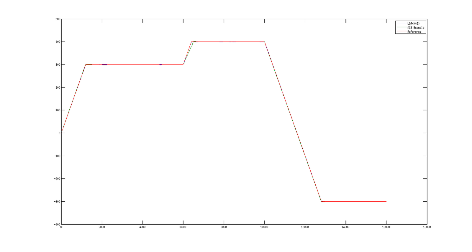
The error between the reference and simulated value using the ac6_example
Rotor speed error
As you can see, in the LQR the error is between 1 and -1.5 which is better than the other controller. Still there are possibilities to reduce the error by increasing the number of the horizon and changing the weight matrices.
Here is another result:
LQR rotor speed error(N=10)
Finally, I can put together the estimator and the controller, so I will end up with the following simulink model:
EKF with LQR
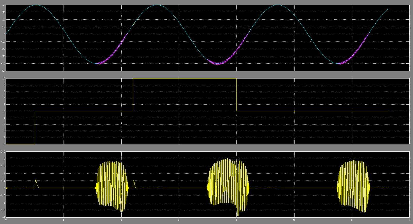
And the result by choosing N=2,


The first subplot is the reference speed and the measured speed, the second is the mechanical torque and the third is the error between the reference and the measured signal.


Monday, October 29, 2012

Dynamic model of a PMSM

The two phase equivalent circuit is widely used to analyse the permanent magnet synchronous machine. In this blog I will present the two phase equivalent circuit of the PMSM dynamic model. 
The three phase electrical dynamic equations can be written as:
$$U_a^S=R_sI_a^S+\frac{d\psi_a^S}{dt}\\U_b^S=R_sI_b^S+\frac{d\psi_b^S}{dt}\\U_c^S=R_sI_c^S+\frac{d\psi_c^S}{dt}\tag{1}$$
where the index $S$ denotes the stator coordinate system.
Also the motor model can be express in the rotating coordinate system
$$U^R=R_sI^R+\frac{d\psi^R}{dt}+j\omega\psi^R\tag{2}$$
Now we can write in the two phase equivalent circuit which is rotating with the same frequency as the rotate magnetic field.
$$u_d=R_sI_d+\frac{d\psi_d}{dt}-\omega\psi_q\tag{3}$$
$$u_q=R_sI_q+\frac{d\psi_q}{dt}+\omega\psi_d\tag{4}$$
where
$$\psi_d=L_dI_d+L_m\tag{5}$$
$$\psi_q=L_qI_q\tag{6}$$
The produced torque can be expressed as:
$$T_e=\frac{3P}{2}\left(L_mI_q+(L_d-L_q)I_d\right)I_q\tag{7}$$
and the motor dynamics can be represented by:
$$T_e=J\frac{d\omega_r}{dt}+B\omega_r+T_L\tag{8}$$ 

Coordinate transformation 

Figure 1. PMSM
As you can see in figure 1, the three phase stationary reference frame can be transformed directly into a two phase reference frame using Park's transformation. Let X represent any of the variables (current, voltage, fluxe), the transformation matrix is given by[4]
$$\left[ \begin{array}{c} X_d \\ X_q \\ X_0 \end{array} \right] =\frac{2}{3} \begin{bmatrix} sin(\theta) & sin(\theta-\frac{2\pi}{3}) & sin(\theta+\frac{2\pi}{3}) \\ cos(\theta) & cos(\theta-\frac{2\pi}{3}) & cos(\theta+\frac{2\pi}{3}) \\ \frac{1}{2} & \frac{1}{2} & \frac{1}{2} \end{bmatrix}\left[ \begin{array}{c} X_a \\ X_b \\ X_c \end{array} \right]\tag{9}$$
The transformation can be a combination of two transformations. First the three phase reference frame can be transformed into a two phase reference frame($abc$ to $\alpha\beta$) by replacing $\theta$ with 0
$$\left[ \begin{array}{c} X_\alpha \\ X_\beta \\ X_0 \end{array} \right] =\frac{2}{3} \begin{bmatrix} 0 & -{\sqrt3\over2} & {\sqrt3\over2} \\ 1 & -{1\over2} & -{1\over2} \\ \frac{1}{2} & \frac{1}{2} & \frac{1}{2} \end{bmatrix}\left[ \begin{array}{c} X_a \\ X_b \\ X_c \end{array} \right]\tag{10}$$
The second transformation is a conversion from stationary to rotating reference frame ($\alpha\beta$ to $dq$)
$$\left[ \begin{array}{c} X_d \\ X_q \\ X_0 \end{array} \right] = \begin{bmatrix}  cos(\theta) & sin(\theta) & 0 \\ -sin(\theta) & cos(\theta) & 0 \\ 0 & 0 & 1 \end{bmatrix}\left[ \begin{array}{c} X_\alpha \\ X_\beta \\ X_0 \end{array} \right]\tag{9}$$

Appendix:

$P$ - Pole pairs
$R$ - Stator phase resistance
$L_m$ - Permanent magnets flux
$B$ - Viscous friction coefficient
$J$ - Inertia
$L_d$ - Direct axis inductance
$L_q$ - Quadrature axis inductance
$\omega$ - Angular velocity

Sources:

  1. Dal Y. Ohm: DYNAMIC MODEL OF PM SYNCHRONOUS MOTORS
  2. Wikipedia: dqo transformation
  3. Mohamed S. Zaky: Adaptive and robust speed control of interior permanent magnet synchronous motor drives
  4. Lecture Set 6.pdf